COMPAS Recidivism#
The COMPAS dataset consists of the results of a commercial algorithm called COMPAS (Correctional Offender Management Profiling for Alternative Sanctions), used to assess a convicted criminal’s likelihood of reoffending. COMPAS has been used by judges and parole officers and is widely known for its bias against African-Americans.
In this notebook, we will use fairlens to explore the COMPAS dataset for bias toward legally protected features. We will go on to show similar biases in a logistic regressor trained to forecast a criminal’s risk of reoffending using the dataset. [1]
[1]:
# Import libraries
import numpy as np
import pandas as pd
import fairlens as fl
import matplotlib.pyplot as plt
from itertools import combinations, chain
from sklearn.linear_model import LogisticRegression

# Load in the 2 year COMPAS Recidivism dataset
df = pd.read_csv("https://raw.githubusercontent.com/propublica/compas-analysis/master/compas-scores-two-years.csv")
df
[1]:
| id | name | first | last | compas_screening_date | sex | dob | age | age_cat | race | ... | v_decile_score | v_score_text | v_screening_date | in_custody | out_custody | priors_count.1 | start | end | event | two_year_recid | |
|---|---|---|---|---|---|---|---|---|---|---|---|---|---|---|---|---|---|---|---|---|---|
| 0 | 1 | miguel hernandez | miguel | hernandez | 2013-08-14 | Male | 1947-04-18 | 69 | Greater than 45 | Other | ... | 1 | Low | 2013-08-14 | 2014-07-07 | 2014-07-14 | 0 | 0 | 327 | 0 | 0 |
| 1 | 3 | kevon dixon | kevon | dixon | 2013-01-27 | Male | 1982-01-22 | 34 | 25 - 45 | African-American | ... | 1 | Low | 2013-01-27 | 2013-01-26 | 2013-02-05 | 0 | 9 | 159 | 1 | 1 |
| 2 | 4 | ed philo | ed | philo | 2013-04-14 | Male | 1991-05-14 | 24 | Less than 25 | African-American | ... | 3 | Low | 2013-04-14 | 2013-06-16 | 2013-06-16 | 4 | 0 | 63 | 0 | 1 |
| 3 | 5 | marcu brown | marcu | brown | 2013-01-13 | Male | 1993-01-21 | 23 | Less than 25 | African-American | ... | 6 | Medium | 2013-01-13 | NaN | NaN | 1 | 0 | 1174 | 0 | 0 |
| 4 | 6 | bouthy pierrelouis | bouthy | pierrelouis | 2013-03-26 | Male | 1973-01-22 | 43 | 25 - 45 | Other | ... | 1 | Low | 2013-03-26 | NaN | NaN | 2 | 0 | 1102 | 0 | 0 |
| ... | ... | ... | ... | ... | ... | ... | ... | ... | ... | ... | ... | ... | ... | ... | ... | ... | ... | ... | ... | ... | ... |
| 7209 | 10996 | steven butler | steven | butler | 2013-11-23 | Male | 1992-07-17 | 23 | Less than 25 | African-American | ... | 5 | Medium | 2013-11-23 | 2013-11-22 | 2013-11-24 | 0 | 1 | 860 | 0 | 0 |
| 7210 | 10997 | malcolm simmons | malcolm | simmons | 2014-02-01 | Male | 1993-03-25 | 23 | Less than 25 | African-American | ... | 5 | Medium | 2014-02-01 | 2014-01-31 | 2014-02-02 | 0 | 1 | 790 | 0 | 0 |
| 7211 | 10999 | winston gregory | winston | gregory | 2014-01-14 | Male | 1958-10-01 | 57 | Greater than 45 | Other | ... | 1 | Low | 2014-01-14 | 2014-01-13 | 2014-01-14 | 0 | 0 | 808 | 0 | 0 |
| 7212 | 11000 | farrah jean | farrah | jean | 2014-03-09 | Female | 1982-11-17 | 33 | 25 - 45 | African-American | ... | 2 | Low | 2014-03-09 | 2014-03-08 | 2014-03-09 | 3 | 0 | 754 | 0 | 0 |
| 7213 | 11001 | florencia sanmartin | florencia | sanmartin | 2014-06-30 | Female | 1992-12-18 | 23 | Less than 25 | Hispanic | ... | 4 | Low | 2014-06-30 | 2015-03-15 | 2015-03-15 | 2 | 0 | 258 | 0 | 1 |
7214 rows × 53 columns
The analysis done by ProPublica suggests that certain cases may have had alternative reasons for being charged [1]. We will drop such rows which are not usable.
[2]:
df = df[(df["days_b_screening_arrest"] <= 30)
        & (df["days_b_screening_arrest"] >= -30)
        & (df["is_recid"] != -1)
        & (df["c_charge_degree"] != 'O')
        & (df["score_text"] != 'N/A')].reset_index(drop=True)

df
[2]:
| id | name | first | last | compas_screening_date | sex | dob | age | age_cat | race | ... | v_decile_score | v_score_text | v_screening_date | in_custody | out_custody | priors_count.1 | start | end | event | two_year_recid | |
|---|---|---|---|---|---|---|---|---|---|---|---|---|---|---|---|---|---|---|---|---|---|
| 0 | 1 | miguel hernandez | miguel | hernandez | 2013-08-14 | Male | 1947-04-18 | 69 | Greater than 45 | Other | ... | 1 | Low | 2013-08-14 | 2014-07-07 | 2014-07-14 | 0 | 0 | 327 | 0 | 0 |
| 1 | 3 | kevon dixon | kevon | dixon | 2013-01-27 | Male | 1982-01-22 | 34 | 25 - 45 | African-American | ... | 1 | Low | 2013-01-27 | 2013-01-26 | 2013-02-05 | 0 | 9 | 159 | 1 | 1 |
| 2 | 4 | ed philo | ed | philo | 2013-04-14 | Male | 1991-05-14 | 24 | Less than 25 | African-American | ... | 3 | Low | 2013-04-14 | 2013-06-16 | 2013-06-16 | 4 | 0 | 63 | 0 | 1 |
| 3 | 7 | marsha miles | marsha | miles | 2013-11-30 | Male | 1971-08-22 | 44 | 25 - 45 | Other | ... | 1 | Low | 2013-11-30 | 2013-11-30 | 2013-12-01 | 0 | 1 | 853 | 0 | 0 |
| 4 | 8 | edward riddle | edward | riddle | 2014-02-19 | Male | 1974-07-23 | 41 | 25 - 45 | Caucasian | ... | 2 | Low | 2014-02-19 | 2014-03-31 | 2014-04-18 | 14 | 5 | 40 | 1 | 1 |
| ... | ... | ... | ... | ... | ... | ... | ... | ... | ... | ... | ... | ... | ... | ... | ... | ... | ... | ... | ... | ... | ... |
| 6167 | 10996 | steven butler | steven | butler | 2013-11-23 | Male | 1992-07-17 | 23 | Less than 25 | African-American | ... | 5 | Medium | 2013-11-23 | 2013-11-22 | 2013-11-24 | 0 | 1 | 860 | 0 | 0 |
| 6168 | 10997 | malcolm simmons | malcolm | simmons | 2014-02-01 | Male | 1993-03-25 | 23 | Less than 25 | African-American | ... | 5 | Medium | 2014-02-01 | 2014-01-31 | 2014-02-02 | 0 | 1 | 790 | 0 | 0 |
| 6169 | 10999 | winston gregory | winston | gregory | 2014-01-14 | Male | 1958-10-01 | 57 | Greater than 45 | Other | ... | 1 | Low | 2014-01-14 | 2014-01-13 | 2014-01-14 | 0 | 0 | 808 | 0 | 0 |
| 6170 | 11000 | farrah jean | farrah | jean | 2014-03-09 | Female | 1982-11-17 | 33 | 25 - 45 | African-American | ... | 2 | Low | 2014-03-09 | 2014-03-08 | 2014-03-09 | 3 | 0 | 754 | 0 | 0 |
| 6171 | 11001 | florencia sanmartin | florencia | sanmartin | 2014-06-30 | Female | 1992-12-18 | 23 | Less than 25 | Hispanic | ... | 4 | Low | 2014-06-30 | 2015-03-15 | 2015-03-15 | 2 | 0 | 258 | 0 | 1 |
6172 rows × 53 columns
Analysis#
We’ll begin by identifying the legally protected attributes in the data. fairlens detects these using using fuzzy matching on the column names and values to a custom preset of expected values.
[3]:
# Detect sensitive attributes
sensitive_attributes = fl.sensitive.detect_names_df(df, deep_search=True)
print(sensitive_attributes)
print(sensitive_attributes.keys())
{'sex': 'Gender', 'dob': 'Age', 'age': 'Age', 'race': 'Ethnicity'}
dict_keys(['sex', 'dob', 'age', 'race'])
We can see that the attributes that we should be concerned about correspond to gender, age and ethnicity.
[4]:
df[["sex", "race", "age", "dob", "age_cat", "decile_score"]].head()
[4]:
| sex | race | age | dob | age_cat | decile_score | |
|---|---|---|---|---|---|---|
| 0 | Male | Other | 69 | 1947-04-18 | Greater than 45 | 1 |
| 1 | Male | African-American | 34 | 1982-01-22 | 25 - 45 | 3 |
| 2 | Male | African-American | 24 | 1991-05-14 | Less than 25 | 4 |
| 3 | Male | Other | 44 | 1971-08-22 | 25 - 45 | 1 |
| 4 | Male | Caucasian | 41 | 1974-07-23 | 25 - 45 | 6 |
fairlens will discretize continuous sensitive attributes such as age to make the results more interpretable, i.e. “Greater than 45”, “25 - 45”, “Less than 25” in the case of age. The COMPAS dataset comes with a categorical column for age which we can use instead.
We can inspect potential biases in decile scores by visualizing the distributions of different sensitive sub-groups in the data. Methods in fairlens.plot can be used to generate plots of distributions of variables in different sub-groups in the data.
[5]:
target_attribute = "decile_score"
sensitive_attributes = ["sex", "race", "age", "dob", "age_cat"]

# Set the seaborn style
fl.plot.use_style()

# Plot the distributions
fl.plot.mult_distr_plot(df, target_attribute, sensitive_attributes)
plt.show()
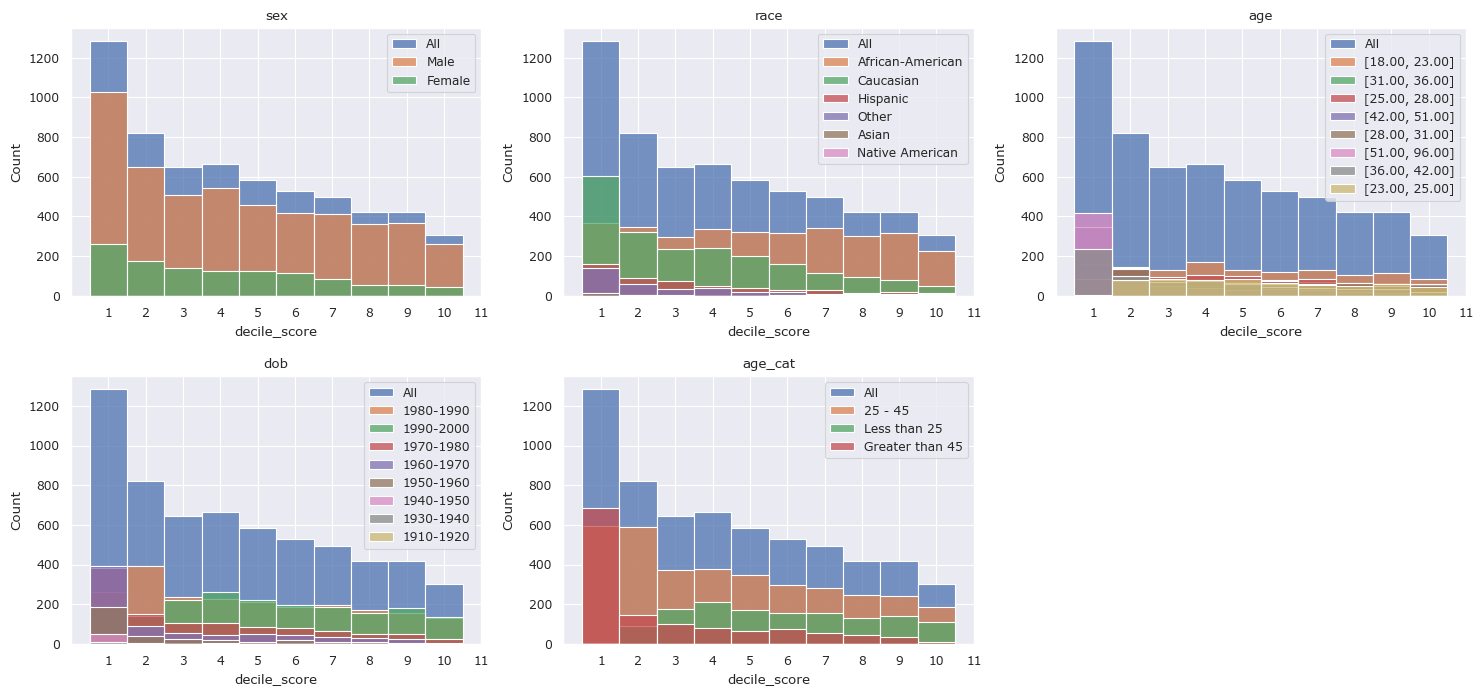
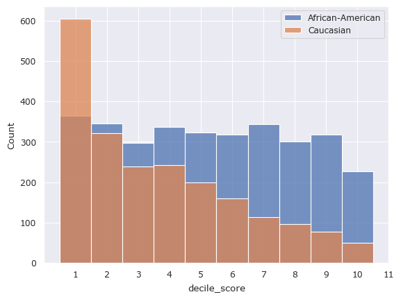
The largest horizontal disparity in scores seems to be in race, specifically between African-Americans and Caucasians, who make up most of the sample. We can visualize or measure the distance between two arbitrary sub-groups using predicates as shown below.
[6]:
# Plot the distributions of decile scores in subgroups made of African-Americans and Caucasians
group1 = {"race": ["African-American"]}
group2 = {"race": ["Caucasian"]}

fl.plot.distr_plot(df, "decile_score", [group1, group2])
plt.legend(["African-American", "Caucasian"])
plt.show()
[7]:
group1 = {"race": ["African-American"]}
group2 = df["race"] != "African-American"

fl.plot.distr_plot(df, "decile_score", [group1, group2])
plt.legend(["African-American", "Rest of Population"])
plt.show()
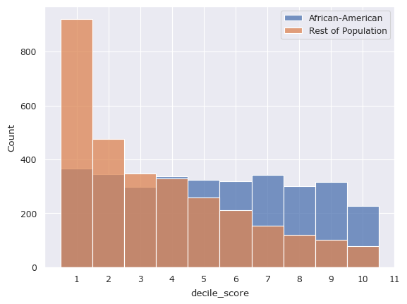
The above disparity by measuring statistical distances between the two distributions. Since the the decile scores are categorical, metrics such as the Earth Mover’s Distance, the LP-Norm, or the Hellinger Distance would be useful. fairlens.metrics provides a stat_distance method which can be used to compute these metrics.
[8]:
import fairlens.metrics as fm

group1 = {"race": ["African-American"]}
group2 = {"race": ["Caucasian"]}

distances = {}
for metric in ["emd", "norm", "hellinger"]:
    distances[metric] = fm.stat_distance(df, "decile_score", group1, group2, mode=metric)


pd.DataFrame.from_dict(distances, orient="index", columns=["distance"])
[8]:
| distance | |
|---|---|
| emd | 0.245107 |
| norm | 0.210866 |
| hellinger | 0.214566 |
Measuring the statistical distance between the distribution of a variable in a subgroup and in the entire dataset can indicate how biased the variable is with respect to the subgroup. We can use the fl.FairnessScorer class to compute this for each sub-group.
[9]:
fscorer = fl.FairnessScorer(df, "decile_score", ["sex", "race", "age_cat"])
fscorer.distribution_score(max_comb=1, p_value=True)
[9]:
| Group | Distance | Proportion | Counts | P-Value | |
|---|---|---|---|---|---|
| 0 | Greater than 45 | 0.322188 | 0.209494 | 1293 | 0.54 |
| 1 | 25 - 45 | 0.042123 | 0.572262 | 3532 | 0.98 |
| 2 | Less than 25 | 0.272500 | 0.218244 | 1347 | 0.53 |
| 3 | Other | 0.253175 | 0.055574 | 343 | 0.69 |
| 4 | African-American | 0.130340 | 0.514420 | 3175 | 0.54 |
| 5 | Caucasian | 0.115572 | 0.340732 | 2103 | 0.64 |
| 6 | Hispanic | 0.184277 | 0.082469 | 509 | 0.67 |
| 7 | Asian | 0.331973 | 0.005023 | 31 | 0.86 |
| 8 | Native American | 0.492532 | 0.001782 | 11 | 0.90 |
| 9 | Male | 0.016210 | 0.809624 | 4997 | 0.97 |
| 10 | Female | 0.068942 | 0.190376 | 1175 | 0.62 |
The method fl.FairnessScorer.distribution_score() makes use of suitable hypothesis tests to determine how different the distribution of the decile scores is in each sensitive subgroup.
Training a Model#
Our above analysis has confirmed that there are inherent biases present in the COMPAS dataset. We now show the result of training a model on the COMPAS dataset and using it to predict an unknown criminal’s likelihood of reoffending.
We use a logistic regressor trained on a subset of the features.
[10]:
# Select the features to use
df = df[["sex", "race", "age_cat", "c_charge_degree", "priors_count", "two_year_recid", "score_text"]]
# Split the dataset into train and test
sp = int(len(df) * 0.8)
df_train = df[:sp].reset_index(drop=True)
df_test = df[sp:].reset_index(drop=True)
# Convert categorical columns to numerical columns
def preprocess(df):
X = df.copy()
X["sex"] = pd.factorize(df["sex"])[0]
X["race"] = pd.factorize(df["race"])[0]
X["age_cat"].replace(["Greater than 45", "25 - 45", "Less than 25"], [2, 1, 0], inplace=True)
X["c_charge_degree"] = pd.factorize(df["c_charge_degree"])[0]
X.drop(columns=["score_text"], inplace=True)
X = X.to_numpy()
y = pd.factorize(df["score_text"] != "Low")[0]
return X, y
df_train = df[:sp].reset_index(drop=True)
# Train a regressor
X, y = preprocess(df_train)
clf = LogisticRegression(random_state=0).fit(X, y)
# Classify the training data
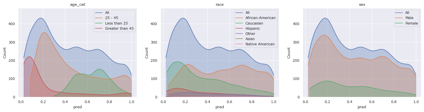
df_train["pred"] = clf.predict_proba(X)[:, 1]
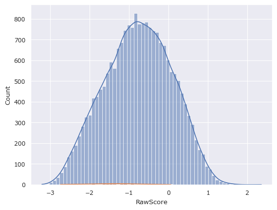
# Plot the distributions
fscorer = fl.FairnessScorer(df_train, "pred", ["race", "sex", "age_cat"])
fscorer.plot_distributions()
plt.show()
[11]:
X = df.copy()
X["sex"] = pd.factorize(df["sex"])[0]
X["race"] = pd.factorize(df["race"])[0]
X["age_cat"].replace(["Greater than 45", "25 - 45", "Less than 25"], [2, 1, 0], inplace=True)
X["c_charge_degree"] = pd.factorize(df["c_charge_degree"])[0]
X.drop(columns=["score_text"], inplace=True)

X.corr()
[11]:
| sex | race | age_cat | c_charge_degree | priors_count | two_year_recid | |
|---|---|---|---|---|---|---|
| sex | 1.000000 | 0.025568 | 0.002701 | 0.061848 | -0.118722 | -0.100911 |
| race | 0.025568 | 1.000000 | 0.104551 | 0.078824 | -0.123963 | -0.088536 |
| age_cat | 0.002701 | 0.104551 | 1.000000 | 0.097368 | 0.169822 | -0.156930 |
| c_charge_degree | 0.061848 | 0.078824 | 0.097368 | 1.000000 | -0.145433 | -0.120332 |
| priors_count | -0.118722 | -0.123963 | 0.169822 | -0.145433 | 1.000000 | 0.290607 |
| two_year_recid | -0.100911 | -0.088536 | -0.156930 | -0.120332 | 0.290607 | 1.000000 |
Above, we see the distributions of the training predictions are similar to the distributions in the data from above. Let’s see the results on the held out test set.
[12]:
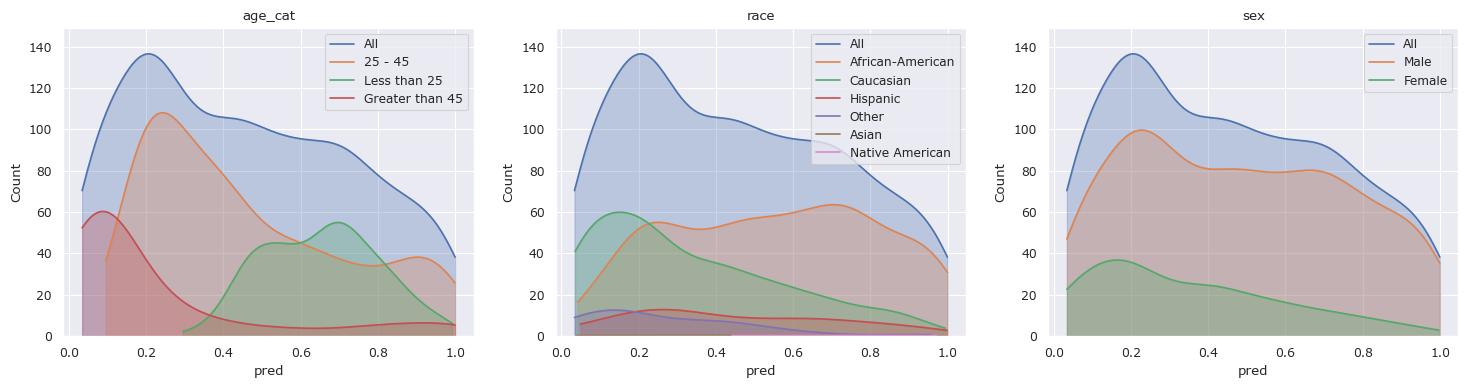
# Classify the test data
X, _ = preprocess(df_test)
df_test["pred"] = clf.predict_proba(X)[:, 1]

# Plot the distributions
fscorer = fl.FairnessScorer(df_test, "pred", ["race", "sex", "age_cat"])
fscorer.plot_distributions()
plt.show()
[13]:
fscorer.distribution_score(max_comb=1, p_value=True).sort_values("Distance", ascending=False).reset_index(drop=True)
[13]:
| Group | Distance | Proportion | Counts | P-Value | |
|---|---|---|---|---|---|
| 0 | Native American | 0.513360 | 0.002429 | 3 | 3.046032e-01 |
| 1 | Greater than 45 | 0.495185 | 0.204858 | 253 | 7.771561e-16 |
| 2 | Less than 25 | 0.456088 | 0.229150 | 283 | 3.005322e-44 |
| 3 | Other | 0.333459 | 0.059109 | 73 | 2.491168e-07 |
| 4 | Asian | 0.238664 | 0.003239 | 4 | 9.366481e-01 |
| 5 | Caucasian | 0.200244 | 0.324696 | 401 | 4.152367e-11 |
| 6 | Female | 0.175752 | 0.208907 | 258 | 3.079097e-06 |
| 7 | African-American | 0.166902 | 0.522267 | 645 | 8.779233e-11 |
| 8 | 25 - 45 | 0.117271 | 0.565992 | 699 | 8.242076e-06 |
| 9 | Hispanic | 0.082636 | 0.088259 | 109 | 4.743583e-01 |
| 10 | Male | 0.046412 | 0.791093 | 977 | 1.830865e-01 |
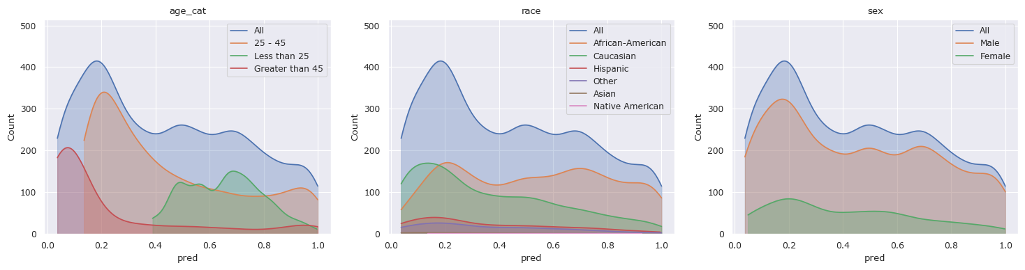
Lets try training a model after dropping “race” from the model and look at the results.
[14]:
# Drop the predicted column before training again
df_train.drop(columns=["pred"], inplace=True)

# Preprocess he data and drop race
X, y = preprocess(df_train)
X = np.delete(X, df_train.columns.get_loc("race"), axis=1)

# Train a regressor and classify the training data
clf = LogisticRegression(random_state=0).fit(X, y)
df_train["pred"] = clf.predict_proba(X)[:, 1]

# Plot the distributions
fscorer = fl.FairnessScorer(df_train, "pred", ["race", "sex", "age_cat"])
fscorer.plot_distributions()
plt.show()
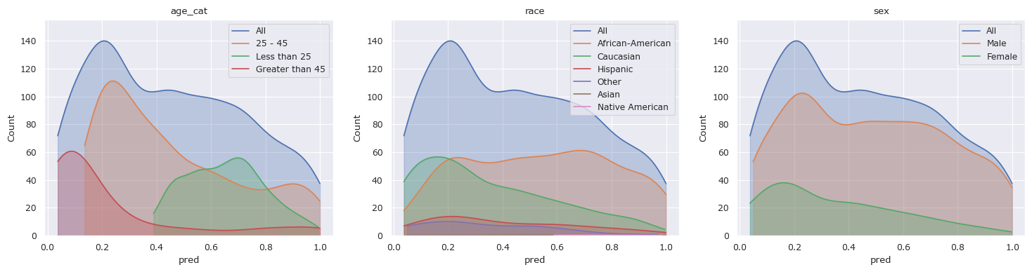
[15]:
# Drop the predicted column before training again
df_test.drop(columns=["pred"], inplace=True)

# Classify the test data
X, _ = preprocess(df_test)
X = np.delete(X, df_test.columns.get_loc("race"), axis=1)

df_test["pred"] = clf.predict_proba(X)[:, 1]

# Plot the distributions
fscorer = fl.FairnessScorer(df_test, "pred", ["race", "sex", "age_cat"])
fscorer.plot_distributions()
plt.show()
[16]:
fscorer.distribution_score(max_comb=1, p_value=True).sort_values("Distance", ascending=False).reset_index(drop=True)
[16]:
| Group | Distance | Proportion | Counts | P-Value | |
|---|---|---|---|---|---|
| 0 | Native American | 0.672065 | 0.002429 | 3 | 7.123637e-02 |
| 1 | Greater than 45 | 0.503900 | 0.204858 | 253 | 7.771561e-16 |
| 2 | Less than 25 | 0.488846 | 0.229150 | 283 | 3.438215e-51 |
| 3 | Asian | 0.243927 | 0.003239 | 4 | 9.240617e-01 |
| 4 | Other | 0.211059 | 0.059109 | 73 | 3.564472e-03 |
| 5 | Female | 0.173141 | 0.208907 | 258 | 4.565218e-06 |
| 6 | Caucasian | 0.160895 | 0.324696 | 401 | 2.577566e-07 |
| 7 | African-American | 0.128776 | 0.522267 | 645 | 1.368363e-06 |
| 8 | 25 - 45 | 0.120753 | 0.565992 | 699 | 3.908314e-06 |
| 9 | Hispanic | 0.097017 | 0.088259 | 109 | 2.824348e-01 |
| 10 | Male | 0.045722 | 0.791093 | 977 | 1.962996e-01 |
We can see that despite dropping the attribute “race”, the biases toward people in different racial groups is relatively unaffected.
References#
[1] Jeff Larson, Surya Mattu, Lauren Kirchner, and Julia Angwin. How we analyzed the compas recidivism algorithm. 2016. URL: https://www.propublica.org/article/how-we-analyzed-the-compas-recidivism-algorithm.